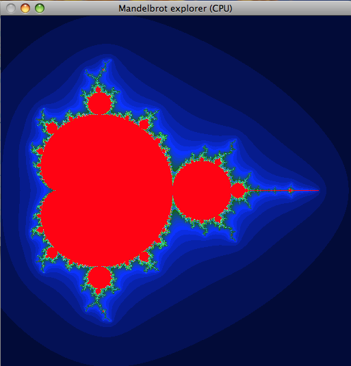
This lab introduces you to CUDA computing with a few small
exercises. We have deliberately avoided larger amounts of code for this
lab, and save that for lab 5.
Some of you have wished to do some of the lab work remotely. This is possible, at least for the parts without graphical output. You ssh to ISY's server ixtab, and from there to one of the Southfork computers.
You can not run on ixtab, since it has no GPU!
So you so like this:
ssh USERNAME@ixtab.edu.isy.liu.se
ssh southfork-06.edu.isy.liu.se
(Or some other Southfork machine. You don't all have to use number 06.)
Note: You should not run remote on a busy machine!
Use the "w" command to see if someone else is logged in.
You should write down answers to all questions and then show us your results.
To be announced. All three labs 4-6 have a common deadline after the
last lab.
To get started, we will use the "simple.cu" example that I introduced in the lecture, arguably the simplest CUDA example. All it does is to assign every element in an array with its index.
Here is the program:
You can compile it with this simple command-line:
nvcc simple.cu -o simple
or, if nvcc is not in your paths,
/usr/local/cuda/bin/nvcc simple.cu -o simple
In Southfork, the path is not set. You can set it with
set path = ($path /usr/local/cuda/bin)
This works nicely in the lab, but for completion, let me show how a slighly more elaborate line can look:
nvcc simple.cu -lcudart -o simple
or
nvcc simple.cu -L /usr/local/cuda/lib64 -lcudart -o simple
Run with:
./simple
(Feel free to build a makefile. You can base it on those from earlier labs.)
If it works properly, it should output the numbers 0 to 15 as floating-point numbers.
As it stands, the amount of computation is ridiculously small. We will soon address problems where performance is meaningful to measure. But first, let's modify the code to get used to the format.
QUESTION: How many cores will simple.cu use, max, as
written? How many SMs?
Allocate an array of data and use as input. Calculate the square root of every element. Inspect the output so it is correct.
To upload data to the GPU, you must use the cudaMemcpy() call with cudaMemcpyHostToDevice.
Note: If you increase the data size here, please check out the comments in section 2.
QUESTION: Is the calculated square root identical to what
the CPU calculates? Should we assume that this is always the case?
Now let us work on a larger dataset and make more computations. We will make fairly trivial item-by-item computations but experiment with the number of blocks and threads.
Here is a simple C program that takes two arrays (matrices) and adds them component-wise.
It can be compiled withgcc matrix_cpu.c -o matrix_cpu -std=c99
and run with
./matrix_cpu
Write a CUDA program that performs the same thing, in parallel!
Start with a grid size of (1, 1) and a block size of (N, N). Then try a
bigger grid, with more blocks.
We must calculate an index from the thread and block numbers. That can look like this (in 1D):
int idx = blockIdx.x * blockDim.x + threadIdx.x;
QUESTION: How do you calculate the index in the array, using 2-dimensional blocks?
In order to measure execution time for your kernels you should use CUDA Events.
A CUDA event variable "myEvent" is declared ascudaEvent_t myEvent;It must be initialized with
cudaEventCreate(&myEvent);You insert it in the CUDA stream with
cudaEventRecord(myEvent, 0);The 0 is the stream number, where 0 is the default stream.
cudaEventSynchronize(myEvent);
Important! You must use cudaEventSynchronize before taking time measurements, or you don't know if the computation has ended!
Finally, you get the time between two events withcudaEventElapsedTime(&theTime, myEvent, laterEvent);where theTime is a float.
You can compile milli.c on the nvcc command-line together with the main program.
Note that in CUDA, large arrays are best allocated in C++ style: float *c = new float[N*N];
Vary N. You should be able to run at least 1024x1024 items.
Vary the block size (and consequently the grid size).
Non-mandatory: Do you find the array initialization time consuming?
Write a kernel for that, too!
QUESTION: What happens if you use too many threads per block?
Note: You can get misleading output if you don't clear your buffers.
Old data from earlier computations will remain in the memory.
Also note that timings can be made with or without data transfers. In a serious computations, the data transfers certainly are important, but for our small examples, it is more relevant to take the time without data transfers, or both with and without.
Note: When you increase the data size, there are (at least) two problems that you will run into:
QUESTION: At what data size is the GPU faster than the CPU?
QUESTION: What block size seems like a good choice? Compared to what?
QUESTION: Write down your data size, block size and timing data for the best GPU performance you can get.
In this part, we will make a simple experiment to inspect the impact of memory coalescing, or the lack of it.
In part 2, you calculated a formula for accessing the array items based on thread and block indices. Probably, a change in X resulted in one step in the array. That will make data aligned and you get good coalescing. Swap the X and Y calculations so a change in Y results in one step in the array. Measure the computation time.
Note: The results have varied a lot in this exercise. On my 9400, I got a very significant difference, while this difference is not quite as big in the lab. This is expected since the lab GPUs are newer. However, lack of difference can be caused by erroneous computation, so make sure that the output is correct.
QUESTION: How much performance did you lose by making data accesses non-coalesced?

Put in a timer in the code. Experiment with the iteration depth.
Also try with double precision. For doing that, you need to specify
-arch=sm_30 on the command-line.
Here you may need one more CUDA event call: cudaEventDestroy(), to
clean up after a CUDA event and avoid memory leaks.
QUESTION: When you use the Complex class, what modifier did you have to use on the methods?
QUESTION: In Lab 1, load balancing was an important issue. Is that an issue here? Why/why not?